Reverse Geocoding in Power BI (and not forgetting Puerto Rico)

Introduction

I solved several pain points recently and decided to put them all together in a single file to share and keep for my own future reference, these pain points are:

• Reverse geocoding coordinates to create a choropleth map
• Creating an AlbersUSA map and including Puerto Rico
• Adding points to a choropleth map
• Cross-highlighting Vega custom visuals

These pain points were solved mostly with Vega in Power BI, with a little help from Python.

Reverse Geocoding with Python

A chloropleth, or filled map, lets us fill the boundaries of a map (like a state or county) with different shading or coloring to indicate the value of a variable.

Imagine you have a dataset which includes latitude and longitude coordinates for any number of things, like cities named Washington (there are 88 in the US), or in the case of this post Costco locations.

If you have an address and want to create a map at the state level, this is pretty easy, but if you want to create a map at the county level or any other unique topology things start to get complicated fast. Imagine manually looking up 600 or more coordinates to determine what county, congressional district, or other organization they lie in. Another potential issue is that the map file you use may not use the same id variable that is available elsewhere.

Reverse geocoding allows us to lookup where a point falls on a map file and return associated parent variable.

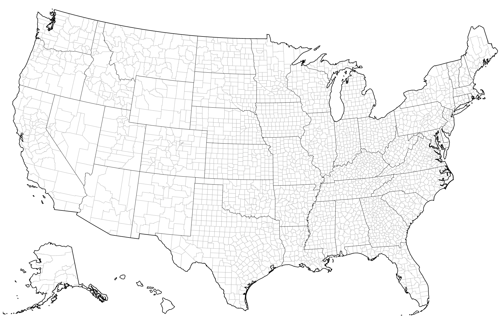
In this case I am using a topojson of US counties and looking up the id (or fips code):

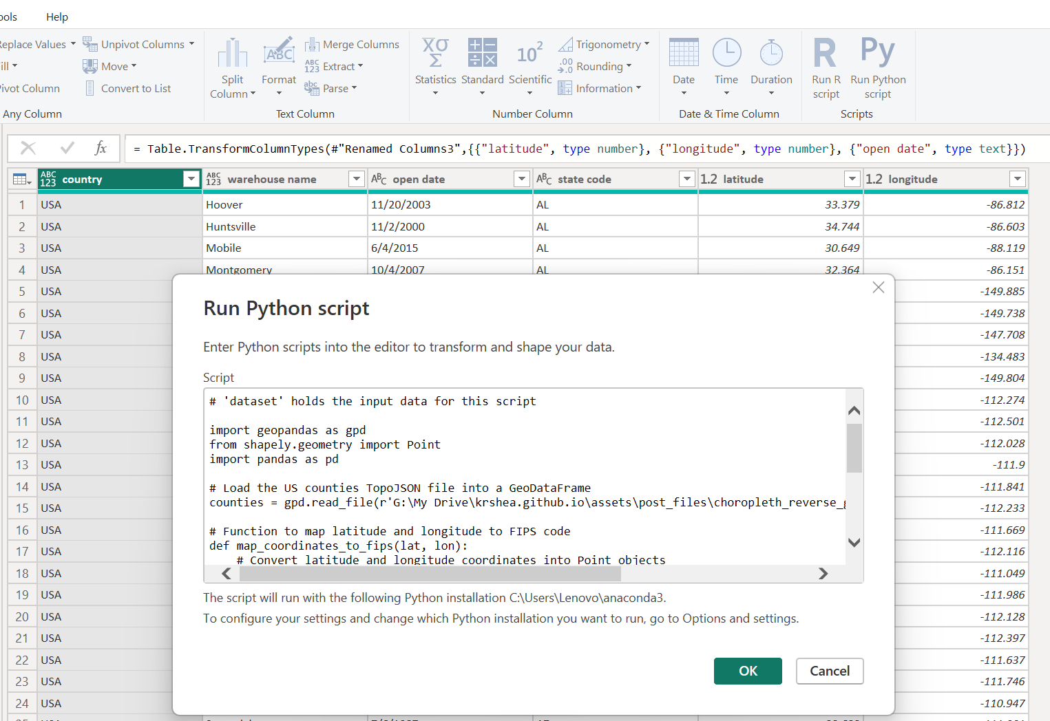
Here is a snapshot of running the Python code in Power Query. If this were a production project I would make this transformation further upstream,but the convenience can’t be denied when protyping things.

# 'dataset'from power query (automatically created) holds the input data for this script
import geopandas as gpd
from shapely.geometry import Point
import pandas as pd

# Load the US counties TopoJSON file into a GeoDataFrame
counties = gpd.read_file(r'G:\My Drive\krshea.github.io\assets\post_files\choropleth_reverse_geocode\counties-10m.json', driver='TopoJSON')

# Function to map latitude and longitude to FIPS code
def map_coordinates_to_fips(lat, lon):
    # Convert latitude and longitude coordinates into Point objects
    point = Point(lon, lat)
    
    # Perform join to find the matching county polygon
    match = counties.contains(point)
    
    # Get the fips code of the matched county
    fips_code = counties[match]['id'].values[0] if any(match) else None
    
    return fips_code

# Map coordinates to FIPS codes and append to the DataFrame
dataset['fips_code'] = dataset.apply(lambda row: map_coordinates_to_fips(row['latitude'], row['longitude']), axis=1)

Disclaimer: I did have to manually map one store location using this methodology, which can be seen if you dig into the pbi file. It seems that my topojson may not have the resolution to capture the little peninsula this Costco is on. Still I think 1/600+ isn’t a bad deal.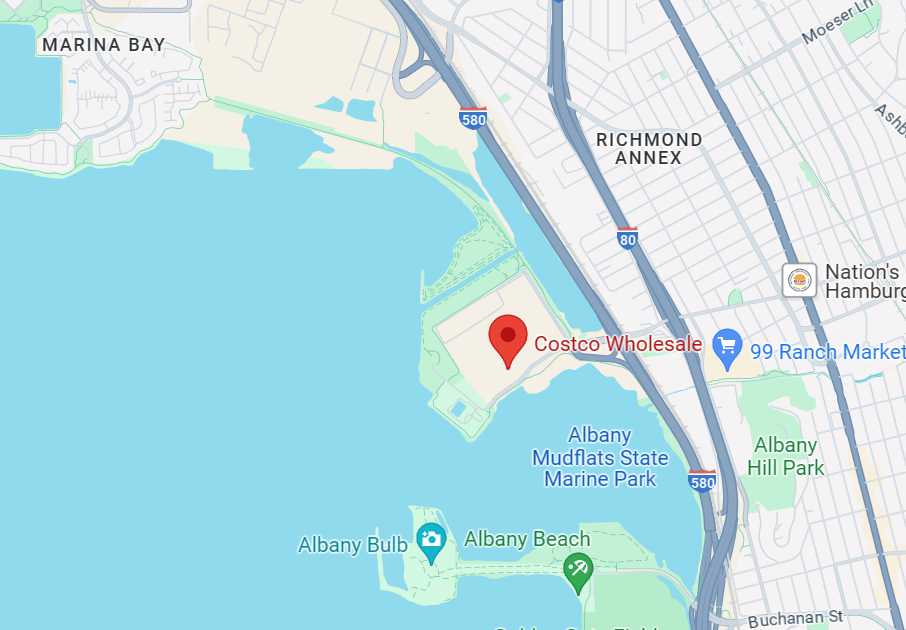

No te olvides de Puerto Rico

What’s missing here?:

When you were a kid did you think Alaska was south of California (right next to Hawaii)? You can thank the AlbersUSA projection, which is the most common projection of the US that allows us to look at each state on a smaller map canvas. Puerto Rico may not be a state, but I think la isla del encanto deserves the same spotlight don’t you? Especially since I have data that needs to be plotted there.

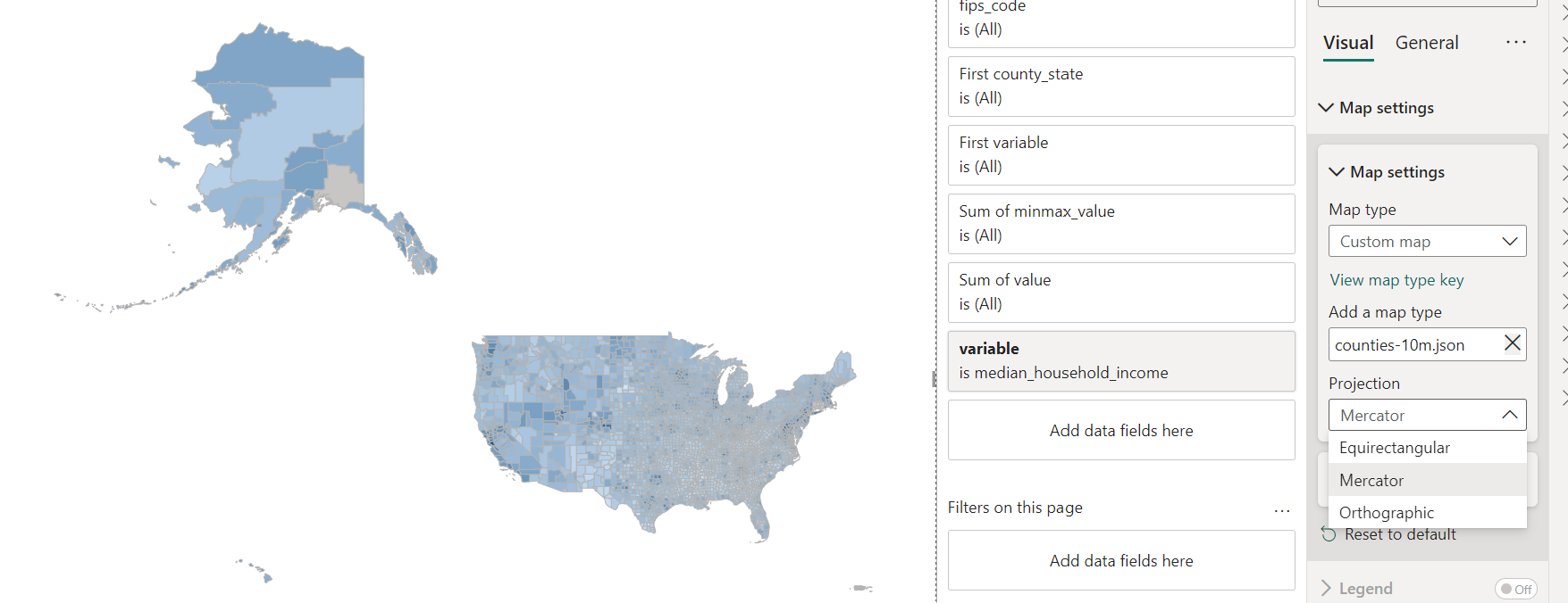
Power BI has a shape map visual in preview status which allows the uploading of topojson files, but it did not allow using the AlbersUSA projection with this particular topojson and I’ve found it to make my workbooks painfully slow when loading county level data.

#Vega to the rescue:

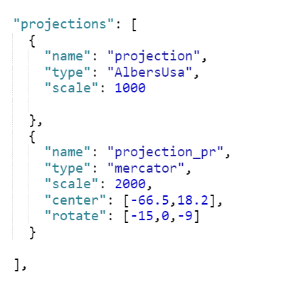
In the same specification in Vega, and using the same data, multiple projections can be defined:

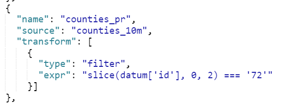
We can also filter our topojson:

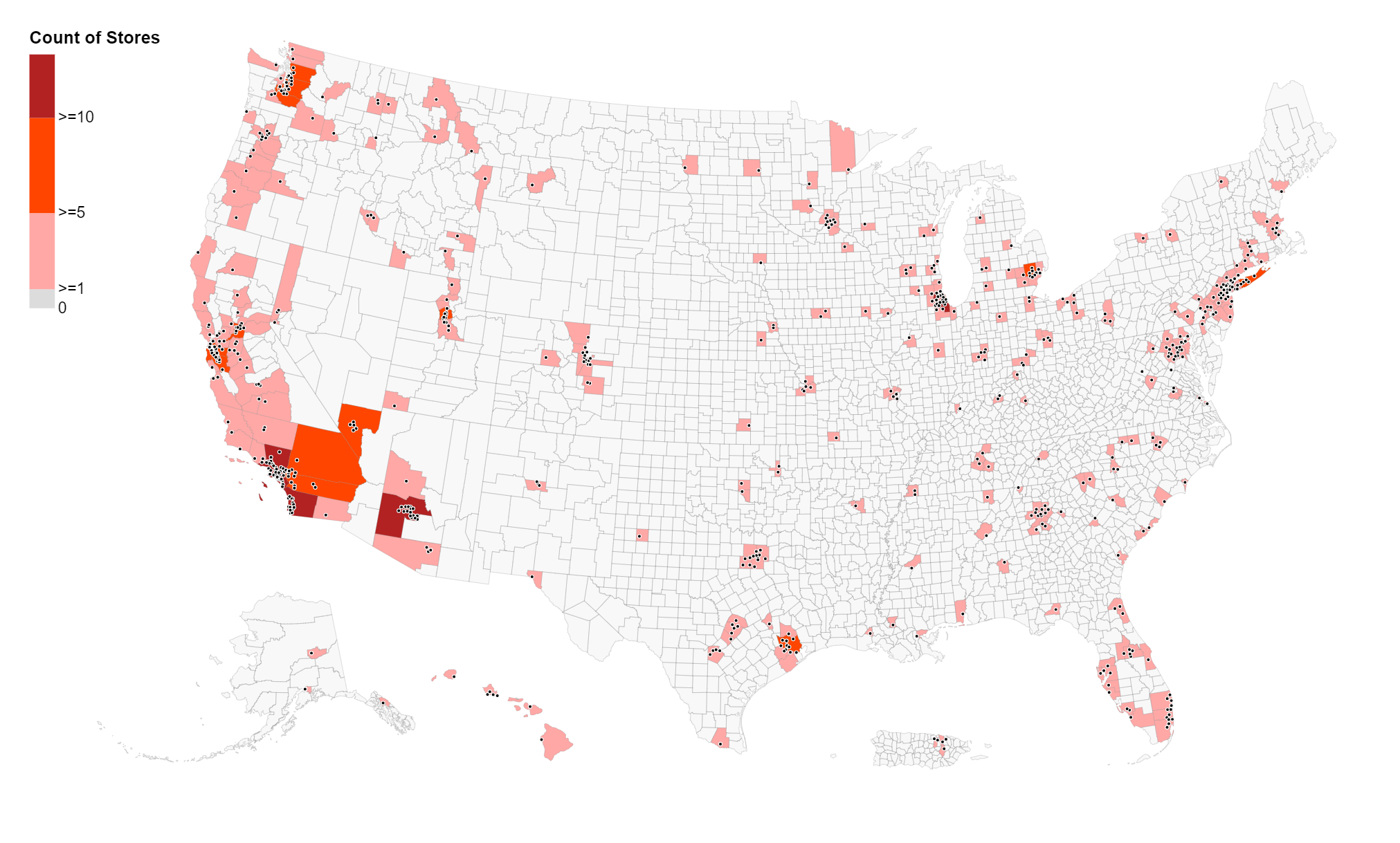
Using the filtered topojson and Puerto Rico projection, we can draw a new layer on top of our AlbersUSA projection:

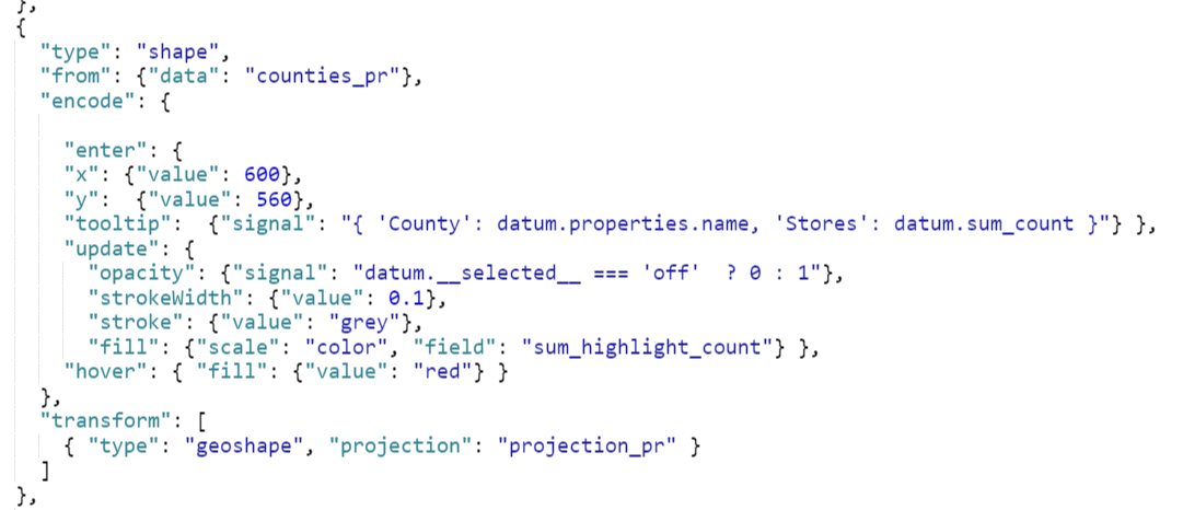
Is Puerto Rico too big here? Maybe, but Puerto Rico has 78 counties (Florida has 67 for comparison). Any smaller and the counties would be invisible, and maybe Puerto Rico deserves some extra spotlight after being left off AlbersUsa maps for so long.

Points on a Choropleth

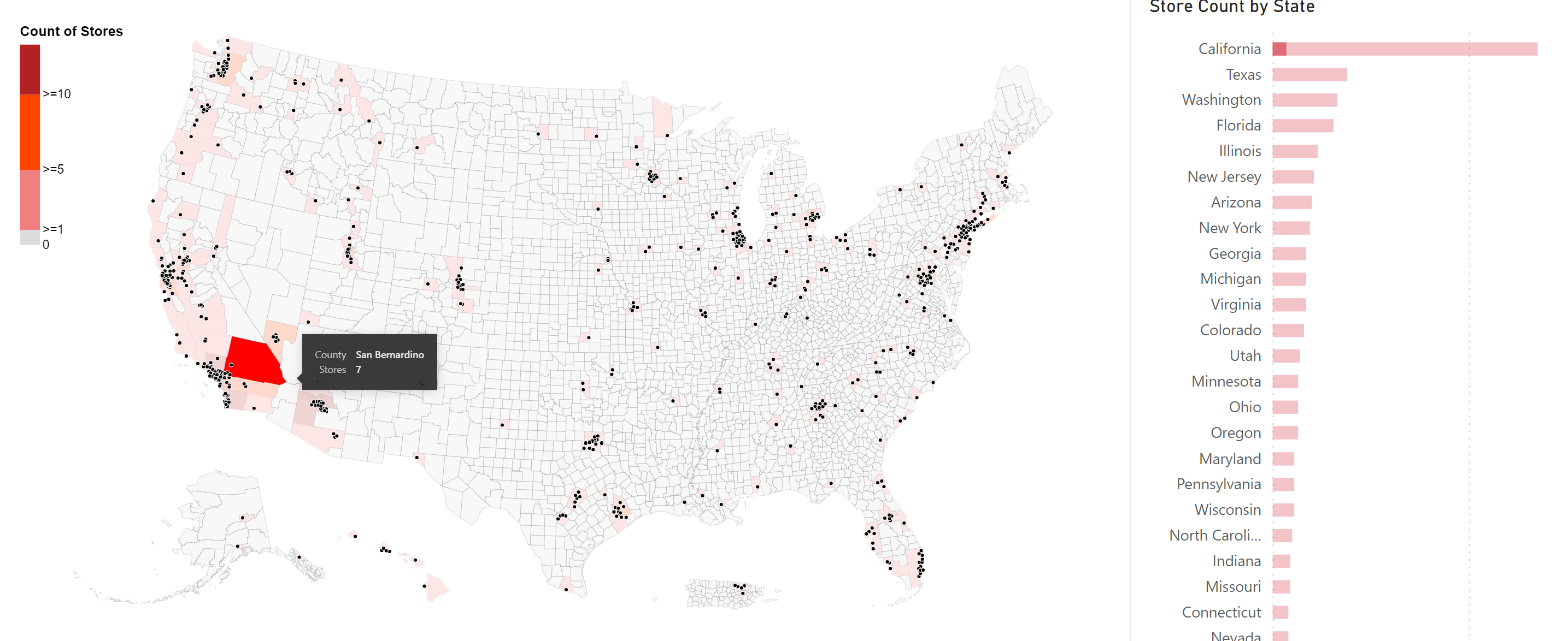
Personally I don’t think these points look great (see the thumbnail for this post), but this was a challenge I gave myself since it’s something I’ve tried to accomplish in the past, and I’ve seen some Power BI thought leaders lamenting that Power BI has no visual that can create choropleths with geo-points overlaid. I recently saw a solution solving this problem by layering two Azure maps visuals on top of each other and playing with opacity, but I think this is a better solution if your organization allows custom visuals.

I will elaborate more on this later, as the key here was mostly on the data prep side, as long as your data is shaped correctly Vega handles this quite easily with layering.

Bonus: Cross-Highlighting Vega Visuals

More on this later, but the downloadable file does have working cross-highlighting in both directions. The Deneb documentation kind of says enter at your own risk. I had to do several lookups and groupings in Vega to get this to work, but the result works great and I find it signficantly faster than the preview shape file visual.

Here is an example of the cross-highlighting in action:

The Download

Here is the Power BI file.

The Vega Code

{
  "$schema": "https://vega.github.io/schema/vega/v5.json",
  "width": 300,
  "height": 300,
  "padding": 0,
  
  "projections": [
    {
      "name": "projection",
      "type": "AlbersUsa",
      "scale": 1000
      
    },
    {
      "name": "projection_pr",
      "type": "mercator",
      "scale": 2000,
      "center": [-66.5,18.2],
      "rotate": [-15,0,-9]
    }

  ],

   "data": [
    {"name": "dataset"},
     {"name": "dataset_grp",
      "source": "dataset",
      
      "transform": [
        {
          "type": "aggregate",
          "groupby": ["id"],
          "fields": ["count","count__highlight"],
          "ops": ["sum","sum"],
          "as": ["sum_count","sum_highlight_count"]
        }
      ]},

    {
      "name": "counties_10m",
      "values": {"TOPOJSON GOES HERE"}
,
        "format": {
          "type": "topojson",
          "feature": "counties"
        },
          "transform": [
        { "type": "lookup", "from": "dataset_grp", "key": "id", "fields": ["id"], "values": ["sum_count"], "default": 0 },
        { "type": "lookup", "from": "dataset_grp", "key": "id", "fields": ["id"], "values": ["sum_highlight_count"] },
        { "type": "lookup", "from": "dataset", "key": "id", "fields": ["id"], "values": ["__selected__"] }
      ]
    },
    {
      "name": "counties_pr",
      "source": "counties_10m",
      "transform": [
        {
          "type": "filter",
          "expr": "slice(datum['id'], 0, 2) === '72'"
        }]
    },
    {
      "name": "dataset_pr",
      "source": "dataset",
      "transform": [
        {
          "type": "filter",
          "expr": "slice(datum['id'], 0, 2) === '72'"
        }]
    },
    {
      "name": "dataset_nopr",
      "source": "dataset",
      "transform": [
        {
          "type": "filter",
          "expr": "slice(datum['id'], 0, 2) !== '72'"
        }]
    }
    
  ],
    "scales": [
    {
      "name": "color",
      "type": "threshold",
      "domain": [0,1,5,10],
      "range": [null,"gainsboro", "lightcoral", "orangered","firebrick"]
    }
  ],

  "legends": [
    {
      "fill": "color",
      "orient": "top-left",
      "title": "Count of Stores",
      "encode": {
      "labels": {
        "update": {
          "text": {
           "signal": "datum.value === 0 ? '0' : isFinite(datum.value) && datum.value > 0 ? '>=' + datum.value : null"
          }
        }}}
    }
  ],

  "marks": [
    {
      "type": "shape",
      "from": {"data": "counties_10m"},
      "encode": {
        "enter": { "tooltip":   {"signal": "{ 'County': datum.properties.name, 'Stores': datum.sum_count }"} },
        "update": {
          "opacity": {"value": 0.2},
          "strokeWidth": {"value": 0.1},
          "stroke": {"value": "grey"},
          "fill": {"scale": "color", "field": "sum_count"} },
        "hover": { "fill": {"value": "red"} }
        
      },
      "transform": [
        { "type": "geoshape", "projection": "projection" }
      ]
    },
     {
      "type": "shape",
      "from": {"data": "counties_10m"},
      "encode": {
        "enter": { "tooltip": {"signal": "{ 'County': datum.properties.name, 'Stores': datum.sum_count }"} },
        "update": {
        "opacity": {"signal": "datum.__selected__ === 'off'  ? 0 : 1"},
        "strokeWidth": {"value": 0.1},
        "stroke": {"value": "grey"},
        "fill": {"scale": "color", "field": "sum_highlight_count"} },
        "hover": { "fill": {"value": "red"} }
              },
      "transform": [
        { "type": "geoshape", "projection": "projection" }
      ]
    },
    {
      "type": "shape",
      "from": {"data": "counties_pr"},
      "encode": {
        
        "enter": {
        "x": {"value": 600},
        "y":  {"value": 560},
        "tooltip":  {"signal": "{ 'County': datum.properties.name, 'Stores': datum.sum_count }"} },
        "update": { 
          "opacity": {"value": 0.2},
          "strokeWidth": {"value": 0.1},
          "stroke": {"value": "grey"},
           "fill": {"scale": "color", "field": "sum_count"} },
        "hover": { "fill": {"value": "red"} }
      },
      "transform": [
        { "type": "geoshape", "projection": "projection_pr" }
      ]
    },
    {
      "type": "shape",
      "from": {"data": "counties_pr"},
      "encode": {
        
        "enter": {
        "x": {"value": 600},
        "y":  {"value": 560},
        "tooltip":  {"signal": "{ 'County': datum.properties.name, 'Stores': datum.sum_count }"} },
        "update": { 
          "opacity": {"signal": "datum.__selected__ === 'off'  ? 0 : 1"},
          "strokeWidth": {"value": 0.1},
          "stroke": {"value": "grey"},
          "fill": {"scale": "color", "field": "sum_highlight_count"} },
        "hover": { "fill": {"value": "red"} }
      },
      "transform": [
        { "type": "geoshape", "projection": "projection_pr" }
      ]
    },
     {
      "type": "symbol",
      "from": {
        "data": "dataset_nopr"},
      "encode": {
        "update": {
          "x": {"signal": "scale('projection', [datum['longitude'], datum['latitude']])[0]"},
          "y": {"signal": "scale('projection', [datum['longitude'], datum['latitude']])[1]"},
          "size": {"value": 10},
          "fill": {"value": "black"},
         "strokeWidth": {"value": 0.5},
         "stroke": {"value": "white"}
        }
      }
    },
     {
      "type": "symbol",
      "from": {
      "data": "dataset_pr"},
      "encode": {
        "update": {
          "x": {"signal": "scale('projection_pr', [datum['longitude'], datum['latitude']])[0]", "offset": {"value": 600}},
          
          "y": {"signal": "scale('projection_pr', [datum['longitude'], datum['latitude']])[1]", "offset": {"value": 560}},
          "size": {"value": 10},
          "fill": {"value": "black"},
         "strokeWidth": {"value": 0.5},
         "stroke": {"value": "white"}
        }
      }
    }


  ]
}