Plotting a Center of Gravity: Data Collection

Introduction

In this article I discuss “scraping” $80 data, and replicate the SQL Row_Number and LAG functions as well as a recursive CTE in Power Query.

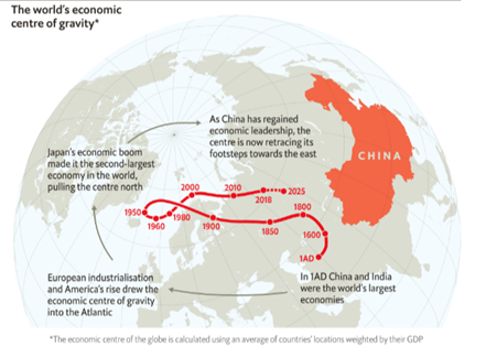
Not long ago I saw a great chart from the Economist showing the world’s economic center of gravity changing over time. Continuing with the theme of maps with time series data on them from my previous post, I thought this kind of chart would tie in great with a project I have been working on related to Costco.

Previously I replicated Charles Joseph Minard’s Napoleon’s march graphic with Vega-Lite, and now I decided to collect some of my own data and try to do something similar to the Economist with Vega, which is a lower level grammar as compared to Vega-Lite. While the data transformations I show here may be more easily accomplished with SQL or Python, my goal is to complete this analysis using Power BI where possible. This post will focus on the data gathering stage of recreating this visual.

US Locations

While admittedly Costco’s center of gravity is certainly less interesting than the World’s Economic Center of gravity, I know there are some Costco superfans out there who may feel differently.

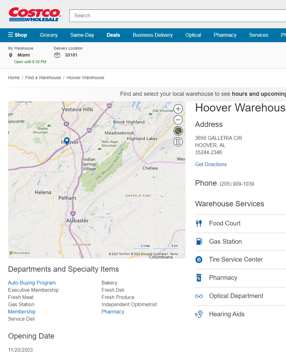
Fortunately Costco.com lists the open date of all of its US stores.

At first I thought I would need to write a Python script to scrape the website, but as I inspected the page source I found that every store location is available as a variable called allWarehouseList. All I needed to do was copy this variable and save as JSON which can be accessed here. A certain data vendor charges $80 for this data by the way, so if you were ever so inclined to buy it, now there’s no need!

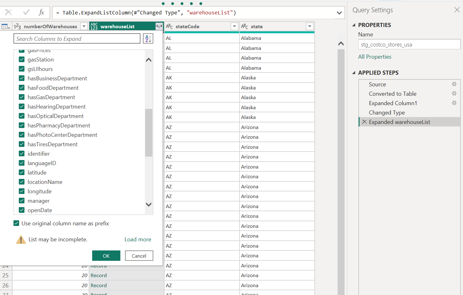
Using Power Query’s JSON connector we can explore the file quite easily, there are a large number of variables available:

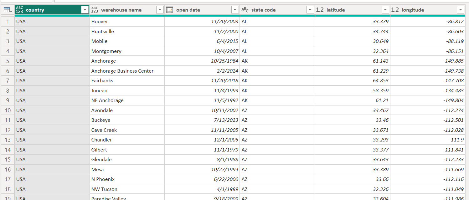
Apply a few more simple transformations and we have a nicely formatted table with the data points I’m interested in:

International Locations

Since I wanted to create a center of gravity chart I thought it would be great to include international stores. One roadblock I ran into was that there is a different website for each country Costco operates in and Costco Canada is the only site which lists store open dates.

Enter the financial statements:

A separate disclosure, although Costco used the equity method in the past to recognize profits from its Mexican stores this isn’t relevant here, just another place to look for the information.

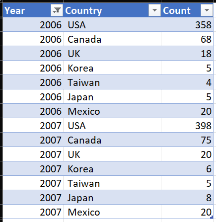
Costco lists store counts each year in the financial statements. The first international location opened in 1985 so that’s 39 years of financial statements that will need to be parsed. As of writing this I’ve gone back to 2001 and organized the data into a table. I will share the data in this post once complete.

Reshaping

So now we have the store counts grouped by year, but our Costco USA data is at the store level, and includes open date, and geographic location.

We need to know the change in international stores from year to year. In SQL I would use the LAG operator, which is not available in Power Query, but we can recreate this easily enough by creating an index or row number for each country and doing a self-join:

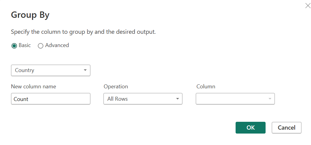
First let’s bring the data into Power Query and group by country using the “All Rows” operation. In SQL terms here we are partitioning the data.

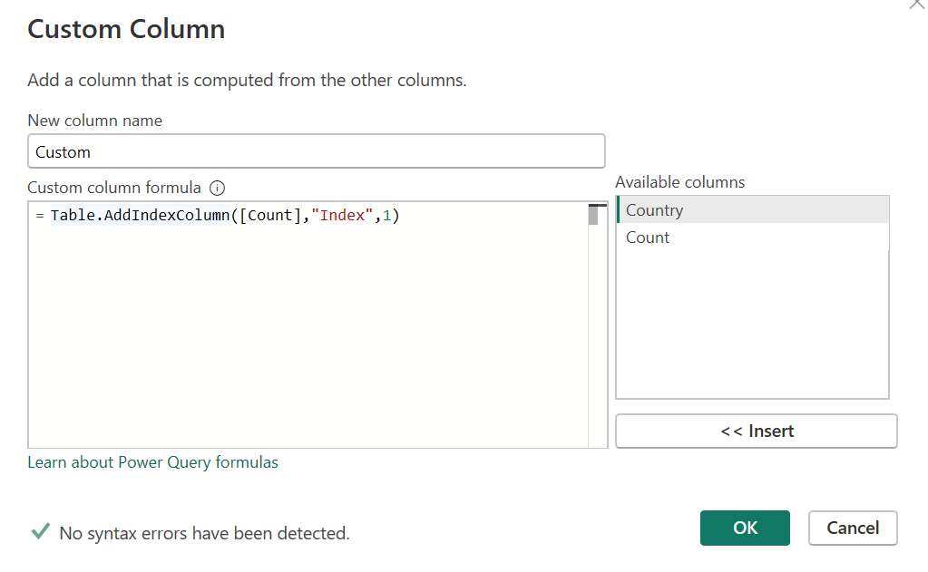
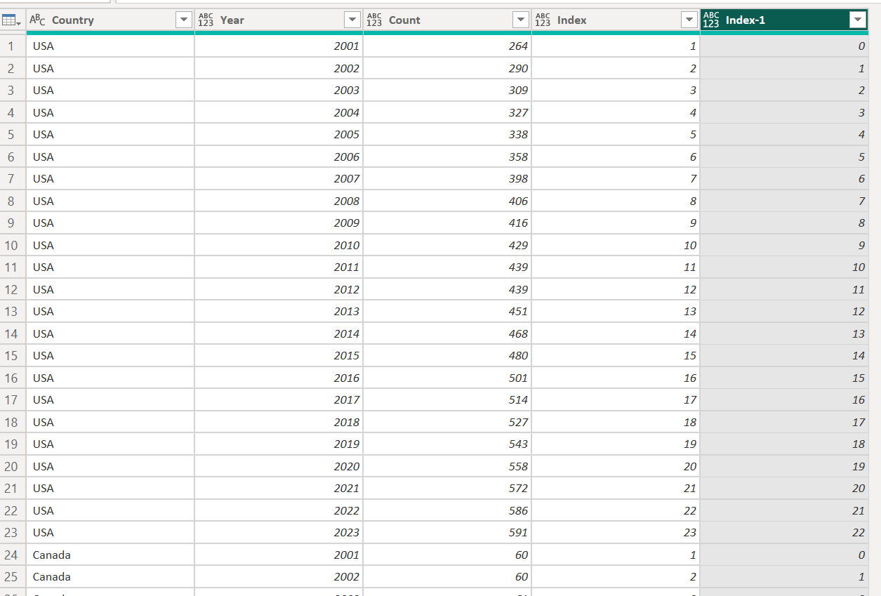
After grouping we add a custom column which will create the row number for each Country.

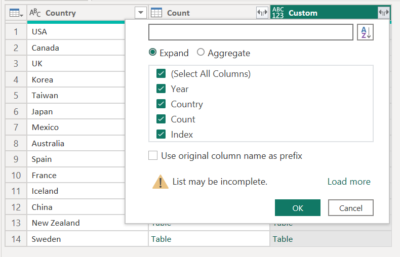
Power Query will store this index as a nested list so we will need to expand it:

Now we have a row number or index partioned by country, to set up the self-join a custom column of Index-1 is added (since we want to replicate LAG).

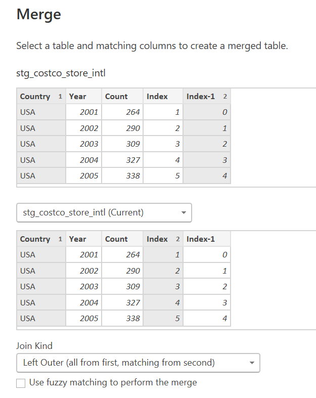
Within Power Query we can merge the table to itself (self-join) using a left outer join to return a null when a country had no stores in the prior year.

After completing our join, removing a few columns and cleaning a couple things up with some very simple transformations our data looks like this. Stores Built is simply the left table value minus the right table value.

Again though, the data is not in the same format as the USA store data. The USA data has one row per store with each’s identifying characteristics. Since we know for example that 2 stores were built in Canada in 2005, in order to match the USA data in shape there should be two rows in 2005 for Canada (and three in 2006, seven in 2007 etc). This can be fixed with a similar technique to creating the group index. By using the List.Repeat function, we can create a nested list for each Country/Year row which contains n number of blank rows. Interestingly in SQL I would do this with a recursive CTE and find the Power Query to be more intuitive, which is rare.

Expanding the list we now two 2018 rows for Korea’s two stores built.

After a few more simple transformations in Power Query we can merge the data with a geographic center table I created (not shown) to return an assumed latitude and longitude of our international store locations (forgive me, my bachelor’s degree is in Economics, I’m a trained assumer).

We now have a dataset that can easily be appended to the USA data:

The next step will be to calculate the geographic center by year in DAX which will be covered in a future post.